Let the data speak!

Battling philosophers: Edwin v Karl

Voice Over: (Michael Palin) 'Boxing Tonight' comes from the Empire Pool, Wembley and features the main heavyweight bout between ET Jaynes, Wayman Crow Distinguished Professor of Physics (cheers; shot of stocky, thick-set Jaynes in his corner with two seconds) And Sir Karl Popper... (shot of Popper’s corner; he is in a dressing-gown with 'Hypothetico-deductivism' on the back; both take off their dressing-gowns as referee calls them together; Sir Karl is wearing a suit underneath) It's the first time these two have met so there should be some real action tonight...

[with apologies to Monty Python]

A simple start

This post concerns “Listening to the data”. I’ll start gently. In 1894, Professor Walter Frank Raphael Weldon (FRS) rolled a set of 12 dice 26,306 times. People had more time then. However, when I see numbers like this, my immediate reaction is one of mild suspicion. Here, there’s nothing to suggest he ended on this strange number for some dark reason.¹ But why not choose a nice round number like 30,000? Did Weldon get tired at this point? Did he lose a die (or his marbles)? Did Florence Weldon (wife and human computer) cry “No more!”? Is there something special about the prime factor 1879?

And no, he didn’t drop dead. At least, not then. This did happen ten years later, at the tender age of 46. Had he lived longer, the whole of 20^th century statistics and indeed ‘Mendelian’ biology might have been different.

Apart from meticulous die-rolling, Weldon had at least two other claims to fame. First, he co-founded the prestigious journal Biometrika together with the grandfather of statistics, Karl Pearson, and nasty eugenicist and racist, Sir Francis Galton. Second, he had a huge fight with the Mendelians, championed by William Bateson. Bateson punted “dominant” and “recessive” genes²; Weldon initially took an opposing view, and in 1906 was just starting to achieve a synthesis, when he contracted pneumonia and died. A pity. Bateson won mainly by default, but the rivalry and bitterness continued.

Goodness of fit

To move on, a question. How would a ‘traditional’ statistician check “goodness of fit?” Back in 1900, when real statisticians often published papers in philosophy journals, Pearson asked “If we have a model that predicts certain numbers, and we have actual measurements, how can we test whether the differences are ‘random’?” His famous solution is the often-used chi-squared test. Carve up the data into manageable chunks, and (with certain assumptions) you can compare not just ‘normal’ distributions of data but a host of off kilter ones too. He showed off his technique using his pal’s dice data. Weldon’s dice were, it seems, loaded. Biased. Not entirely random. Whatever.

But even in that original paper, Pearson warns us. A good fit will still continue to fit smaller samples or more rough grouping; the opposite is not true. Finer divisions or larger numbers may make your “fit” a lot worse. Joseph Berkson, also the father of “Berkson’s paradox”³ underlined that second point: paradoxically, the bigger your study, the more likely the chi-square is going to cry out “this model is false”. This leads us straight into the arms of George Box, often phrased:

Despite his paper on “Science and Statistics” being mostly a huge tribute to Ronald Fisher,⁴ it’s worth a read because Box’s main theme is our familiar feedback loop: Science is iteratively wrong. Don’t fall in love with your model.

All Models are Wrong

We see it again and again. Starting assumptions are hugely important. If you believe you can “listen to your data”, well then—what language are they speaking? What language are you speaking?

We’ve already had a taste of this—in my recent post my naiveté was displayed for all to see. I reasoned that “Bayes is best” (courtesy of Cox’s theorem) and then deduced that because the Bayesian Information Criterion (BIC) is, well, Bayesian, it too should be ‘best’. I was wrong, and the reason I was wrong is very edifying. Bayes’ pretty much assumes that among competing hypotheses, we have the truth!

The stark truth is that we cannot know the truth. This simple observation suggests we should use Bayes carefully, and constrains us to a measure of humility. Our little chi-square exploration is simply a ‘frequentist’ demonstration of something that is completely counter-intuitive. We imagine that bigger studies must be ‘better’.

But we may also have several wins here. A slightly weird one is pointed out by Lindsay and Liu. We can collect sufficient data in order to ensure that our models are false. Then we look backwards, and see how incoherently they performed! For details (and a rabbit hole), read the paper. We’ll explore some other treasure soon. But …

The next few sections might seem intimidating. They are short but intense bouts. The problem is not the maths. I fudge the maths, you see! But there are still a few issues. First, we’re doing a bit of statistical philosophy, which is not everyone’s cup of tea.⁵ But a lot of the ‘philosophy’ is stuff we’ve already done in other posts. I provide helpful links, too. Second we dig fairly deep into solutions to things that you mightn’t consider problems. If you’re struggling—hum along. You’ll soon pick up the tune.

And if you lose it at some point, well then. Skip to the final section. It’s called “Back to the beginning”. There, if you’re now suitably angry, you may want to go back and read the rest more carefully!

Popper

In my very first post on Substack you may see a strange similarity between my take on Science and how Karl Popper conceived it. Yep. I pretty much stole his ‘hypothetico-deductive approach’. Here we know the tune: start with a problem to solve. Make explanatory theories. Test them: test the logic, and test them in the real world. Most will fail—they will be refuted. Those that succeed are not ‘right’ in some absolute sense—they have simply not yet been shown to be wrong. But they can be useful.

But hang on! In my most recent post I enthused about Bayes. Isn’t this just calculating posterior probabilities? A crappy model will be gradually pushed aside by one that just works better—the posterior distributions will change appropriately with the evidence. Won’t it? Who needs refutation? And Bayesians like ET Jaynes have been quite rude about Popper’s approach, haven’t they?

Slugging it out about induction

Popper and Jaynes are both dead. This is unfortunate for several reasons, the main ones perhaps being that Jaynes left his 700-page magnum opus to be finished by his student Larry Bretthorst, and Popper never lived to see our modern take on causality. We have what we have.

One thing we do have is a legacy squabble about induction. What’s ‘induction’? The idea is that we can use ‘inductive methods’ to move from specific, singular statement to universal statements—generalisations about reality. But David Hume pointed out ages ago that past regularities are no guarantee of future regularities. We first have to assume some sort of ‘uniformity’ across our observations, and everything not yet observed. Justifying this assumption universally is a tad problematic. The inverse probability of Bayes is meant to fix all of this—but still makes similar assumptions.

Yet, it’s abundantly clear that Bayes works. We can take a model, acquire useful information, update our model, and make decisions (do things) based on these updates. For example, we used our knowledge of likelihood ratios to choose the best test, in order to almost rule out significant furring up of arteries in the heart.

The rest of this post will explore why the two approaches are not just “not enemies”, but are needed together, if we are to do good science. The boxing image at the start (patched together using Gimp) turns out to be quite inappropriate. Despite some technical disagreements,⁶ Jaynes and Popper fit together unexpectedly well.

Just say “No!”

In a brilliant article published in 2015 in the somewhat obscure British Journal of Mathematical and Statistical Psychology, Andrew Gelman and Sosma Shalizi examine the ‘traditional’ Bayesian take on how to do things. They don’t muck around:

In [the traditional Bayesian] view, the [posterior distribution] p(θ|y) says it all, and the central goal of Bayesian inference is computing the posterior probabilities of hypotheses. Anything not contained in p(θ|y) is simply irrelevant, and it would be irrational (or incoherent) to attempt falsification, unless that somehow shows up in the posterior. The goal is to learn about general laws, as expressed in the probability that one model or another is correct.

...

We think most of this received view of Bayesian inference is wrong [!]

Their paper is worth a read for the real-life examples. I’m going to be a lot simpler.

Box & Jaynes

Gelman and Shalizi first point out that most Bayesians don’t bother to check their models. Why? Here’s where things can become very technical. In contrast, I’m going to try to keep things simple. Here goes ...

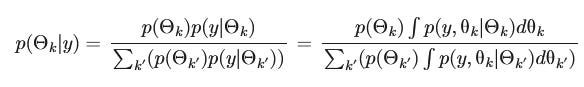
Oh. Woops. Do you see the problem? I’ve just gone full Bayes on you. That’s not fair.

Our first step will be to translate the above small monster—broadly—into English. Very broadly. This is helped by the fact that we’ve already pretty much explained the problem in simple words. I did so in my first post, and then followed up in my Bayes post.

On the left, p(Θ_k|y) refers to the posterior distribution of a set Θ of k models. The rest is just the ‘standard’ Bayesian way of working out those distributions. Shove in a few integrals, Blah, blah. But — we know that none of those models can be shown to be true in any absolute sense! In fact, no reasonable statistician even believes from the start that they are ‘right’. As Gelman and Kumar say:

… it is hard to claim that the prior distributions used in applied work represent statisticians' states of knowledge and belief before examining their data, if only because most statisticians do not believe their models are true, so their prior degree of belief in all of Θ is not 1 but 0.

This has huge implications. The main one is that you must “Science It”—go back and re-examine your most successful (but still false) model. There are even three ways to do this:

1. Check your model by looking for patterns in the ‘error terms’.

2. Walk backwards. You can take your best ‘fitted model’, run simulations, and check that they resemble the original data.

3. Check your fitted model against the data not used during fitting.

All of these are powerful, and all are neglected if you believe that “the truth” is hiding within your model. Fixation on the truth can deceive you into throwing away the many ways you can slay your most cherished model. And fix it—often by expanding it into a better model, using what you’ve just learnt.

We can generalise that last point

You can see that naive generalisation using a Bayesian, inductive approach is rather unwise. Not only are we sure that none of our models is ‘true’, but there are also a few other issues:

1. If you want your calculations to end before the entropic death of the universe, then you often can’t include everything that might be relevant. There are always computational tradeoffs. There are known factors we often exclude or fudge. And (Box again) “overelaboration and overparameterisation is often the mark of mediocrity”.

2. We can’t possibly know what “unknown unknowns” are lurking out there. In the Box paper above, he describes how Fisher was perplexed. A lot of Fisher’s initial analyses looked at shit spread over agricultural plots. After about 1870, there was an unaccounted, slow decrease in agricultural yield. After much deliberation, Fisher decided that the problem was overgrowth of the slender foxtail grass Alopecurus. He blames the Education Act of 1876—little boys were no longer in the fields, pulling out this weed.⁷

3. There is no way of knowing a priori what unconscious biases you’ve introduced into your model.

We’ve already had a taste of this last point with our recent causal models. If you condition on the wrong factors, then you open up back doors and see causes that aren’t there. If you fail to condition on a confounder, then you underestimate causes that are there.

Or as ET Jaynes himself put it:

Put more strongly, it is only when our inductive inferences are wrong that we learn new things about the real world. For a scientist, therefore, the quickest path to discovery is to examine those situations where it appears most likely that induction from our present knowledge will fail.

Here’s how I like to conceptualise things.⁸

We cannot know where our most loved theories are egregiously wrong. There is a border of belief, which is continually being refashioned by Science. The method we use to ‘Science it’ is, for want of a better term, hypothetico-deductive. Popper’s playground. Within the shifting compass of our models, Bayes rocks.

Back to the beginning

Which brings us back to the start. It’s easy. We can’t “let the data speak”. The data are mute. Models need to be fixed and this is an active process—doing Science—rather than sitting back and passively waiting for Bayes to work miracles!

At this point I’d love to talk about two things, Pearl’s causal hierarchy, and (naturally) receiver operating characteristic curves. Both are inviting, but before we go there, my next post will be devoted to randomness, which only seems a simple concept. Entropy might get sucked into the vortex, too. We’ll even build our own, physical random number generator.

My 2c, Dr Jo.

1. In contrast, Italian mathematician Mario Lazzarini tossed a needle onto a grid 3,408 times and claimed to have determined a value of pi accurate to six decimal places. This was based on (a) Buffon’s needle problem and (b) flagrant cheating.

2. We then confuse things by talking about ‘incomplete penetrance’, ‘Lyonisation’, ‘mosaicism’ and ‘epigenetic factors’. Which are not bad terms, but do mess with the heads of people brought up on the “lies to children” of recessive | dominant. It’s also highly likely that Mendel subconsciously fudged his findings—his results are too perfect. Again, this doesn’t make them wrong, but it does temper our enthusiasm for lies to children. Hindsight is a terrible thing.

3. Berkson’s paradox is tricky, but we already know how to deal with it. Let’s say talent and attractiveness aren’t correlated in the whole population, but if you only examine celebrities—who must have some combination of the two—then the two become negatively correlated. From a causal point of view we open up a back door because there’s a collider here: a causal arrow goes from both talent and attractiveness to celebrity.

And here’s his chi-square comment:

I make the following dogmatic statement, referring for illustration to the normal curve: “If the normal curve is fitted to a body of data representing any real observations whatever of quantities in the physical world, then if the number of observations is extremely large—for instance, on the order of 200,000—the chi-square P will be small beyond any usual limit of significance.

If this be so, then we have something here that is apt to trouble the conscience of a reflective statistician using the chi-square test. For I suppose it would be agreed by statisticians that a large sample is always better than a small sample. If, then, we know in advance the P that will result from an application of a chi-square test to a large sample there would seem to be no use in doing it on a smaller one. But since the result of the former test is known, it is no test at all!

For a Bayesian take on all of this, see Chapter 9 of Jaynes’ Probability Theory: the Logic of Science.

4. Fisher had his flaws, including acting as a shill for tobacco companies in later life, and malevolently and relentlessly persecuting people who didn’t toe the line with his particular take on statistics. Box is too nice. He also doesn’t actually say the words “All models are wrong but some are useful”, but his comments on the scientific method as an antidote to ‘cookbookery’ (forcing problems into molds) and ‘mathematistry’ (maths for maths’ sake) are even more pertinent today:

In such areas as sociology, psychology, education, and even, I sadly say, engineering, investigators who are not themselves statisticians sometimes take mathematistry seriously. Overawed by what they do not understand, they mistakenly distrust their own common sense and adopt inappropriate procedures devised by mathematicians with no scientific experience.

5. Unless you’re Muriel Bristol.

6. Jaynes criticised Popper appropriately when Popper was wrong about his ‘propensity interpretation’; it would seem Popper didn’t understand the utility of Bayesian ‘induction’, but he was in turn quite right about abuse of induction. The first round is 10-10.

7. Alopecurus myosuroides is notoriously herbicide resistant. I have this strange premonition that not a few right-wing politicians (who hark back to the old days with fondness) would see this as justification for getting children with their small hands back into the fields!

8. Otherwise known as “Do Deformed Rabbit. It’s my favourite.”