Why we fail
An explosion of quackery: Part IV

Human beings seem uniquely vulnerable to quackery.⌘ But are they? In the following, we’ll explore whether other hominids like the chap above might have similar failings. Even pigeons may not fare well. I’ll also put forward a fairly easy explanation for why we fail: we’re vulnerable.
Dr Holmes sets the scene
A medicine—that is, a noxious agent, ... should always be presumed to be hurtful. It always is directly hurtful; it may sometimes be indirectly beneficial. [...] Throw out opium, which the Creator himself seems to prescribe, for we often see the scarlet poppy growing in the cornfields, as if it were foreseen that wherever there is hunger to be fed there must also be a pain to be soothed; throw out a few specifics which our art did not discover, and it is hardly needed to apply; throw out wine, which is a food, and the vapors which produce the miracle of anaesthesia, and I firmly believe that if the whole materia medica,1 as now used, could be sunk to the bottom of the sea, it would be all the better for mankind,—and all the worse for the fishes.
Oliver Wendell Holmes Sr. Massachusetts Medical Society address, 30 May 1860
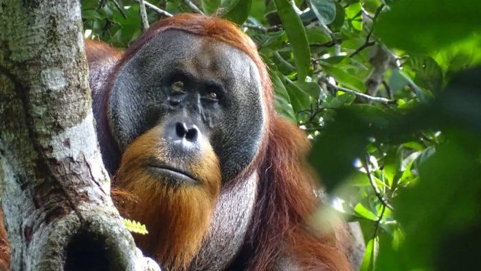
Recent evidence suggests that even apes apply poultices and take substances that might be therapeutic. This naturally invites several questions, so let’s look at the very special orangutan pictured above. He’s ‘Rakus’, a dominant (‘flanged’) adult male.
‘Orangutan takes medicine’
I recently read a paper in Nature scientific reports titled “Active self-treatment of a facial wound with a biologically active plant by a male Sumatran orangutan”. The authors claim that this is the first report of active wound treatment ...
“… with a plant species known to contain biologically active substances by a wild animal”.
You may have spotted the healed wound beneath the right eye of the ape2 in question.
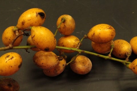
The authors do rather bang on about the plant in question—Fibraurea tinctoria—noting that this obsolete yellow dyestuff has been used as a traditional medicine for “analgesic, antipyretic, antidote, and diuretic effects”, and then rhapsodising about furanoditerpenoids and protoberberine alkaloids (mostly palmatine but also jatrorrhizine and columbamine). There are a few problems here.
Why this is wrong
Ironically, it seems that the authors of this prestigious article seem to have fallen prey to the very problem we’re investigating—belief in the healing power of herbs!
First up, they freely admit this is an unusual behaviour, not seen before in thousands of hours of observation of orangutans. How do they determine that the orangutan deliberately sought out a ‘healing herb’, rather than just chewing something warm and wet and slapping it on to ease the irritation, in much the same way that another animal might lick a wound? Is this just sophisticated wound licking?
There are further issues. From one observation, they seem to be drawing a rather long bow—orangutans creating a pharmacopoeia with at least one ‘traditional medicine’. We’ll get back to this issue below.
But an even bigger problem is their naive acceptance that (a) this herb has healing properties; and (b) that at least one orangutan worked this out. As we saw with William Withering,⌘ it’s rather difficult to tease out whether a ‘herb’ is beneficial, in addition to the harms it causes. Given my exploration⌘ of Aristolochia, which found its way into a huge number of herbal medicines despite causing kidney failure and cancer, even humans are not that hot at teasing out benefits.3 But perhaps the orangutan just believes?
Remember Holmes’ caution. So how do the healing claims here stack up?
Jatrorrhizine, which features prominently in traditional Chinese medicine, has had glowing reviews. There are so many claimed benefits. But where are the toxicity data? Is it safe? Where are the clinical trials showing benefit? Before you rush out and invest in Fibraurea poultices, note that its main component palmatine kills cells and damages DNA. Oops.4
Healing behaviour?
This ‘healing herb’ scenario seems sketchy. But what about other examples? The late Jane Goodall noticed that chimpanzees eat leaves, and subsequent work suggested this eliminates intestinal parasites, at least some of the time. Perhaps other hominid ‘cultures’ actually do pass on knowledge?
We humans do this. We’ve done it for millennia. I’ve previously commented⌘ (footnote 4) on the presence of digitalis glycosides in the arrows of hunters from Southern Africa at least 7000 years old, and the likelihood that this extends back for 50,000 years or more.
There are a few problems with this extrapolation, though. Most obvious is that humans have complex languages that allow us to transmit detailed information about cultural artefacts. But more than this, things like arrow poisons—things that actually work reliably—occupy a central position in cultures where they are used, because of the high rewards and high risks.
When tempers rise and violence threatens, friends and relatives go find the poisoned arrows and hide them far away in the bush.5
In contrast, it seems to me that a lot of apparent ‘therapeutic’ use of ‘herbs’ by other primates may simply be like cats eating grass. This activity may be favoured by natural selection because eating grass (and foliage, and seeds) helps animals to expel intestinal parasites, increasing muscle activity in the digestive tract.6
Pigeon religion!
I’ve previously commented⌘ on BF Skinner’s finding that when confronted with entirely random rewards, pigeons would acquire and reinforce ‘superstitious’ behaviours. Why should this be?
The answer might well lie in decision theory. The problem we (or the pigeon, or the orangutan) are faced with is teasing out the ‘true positives’ from the ‘false positives’. There’s a balance here. If you startle every time the play of shadows on the leaves suggests the presence of a lurking leopard, you may waste a lot of energy jumping at shadows, but this is likely nothing compared to the inconvenience (and dearth of descendants) that occurs if you’re eaten by a real live leopard.
The boy who cried leopard
There are different sorts of test. But even if the test is great, we still need to establish a threshold, above which we act. Imagine a test of “leopardness” on a scale of say 0–10, and a tribe of skilled proto-humans walking through the bush. They have different thresholds for crying ‘leopard’. There are shadows all around. Some contain leopards.
Let’s formalise this. Those who are sensitive are more jumpy, but may miss fewer leopards; those who are specific will be pretty sure when they see one, but will unfortunately miss several leopards—and missing one is often enough.
We say that a sensitive test that is negative rules out the condition (sometimes abbreviated to SnNout); a specific test that is positive rules it in (SpPin). We might even measure this. Imagine a graph with ‘leopardness’ on the X axis, and ‘number of shadows’ for Y.
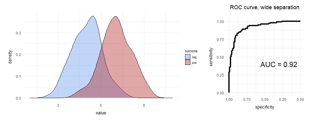
We draw two curves. The blue curve represents situations where there are just shadows, and no leopards; for the red curve, the shadows contain leopards. At a given leopardness, we set a single threshold, cutting each curve in two.
For the red curve ‘true positive fraction’ (TPF, sensitivity) is the proportion of true leopard shadows above the cutoff; the ‘false negative fraction’ (FNF) is those we missed. Similarly, for blue, the TNF is leopardless shadows below the cutoff; the important false positive fraction (FPF) is where we’re jumping at shadows. We define ‘specificity’ as one minus the FPF (that is, the TNF). And here are your curves:
ROC and roll
I pseudorandomly generated these data. Leopards are our outcome here, but we can do exactly the same thing for say, a lab test for heart failure or for a heart attack, or teasing out whether a something detected using radar represents ‘enemy’ or ‘noise’.7
The above is a really good test. There’s decent separation—but there’s still some overlap. One way of characterising that overlap is to construct the receiver operating characteristic curve on the right. Let’s build a ROC curve.
Draw a square. The Y axis is the sensitivity (TPF). Smart spotters of leopards and other things will already have noticed that in the diagram, the X axis runs from one to zero. This is because we’ve labelled it ‘specificity’. Alternatively, you could use FPF, and run from 0.0–1.0. Same difference.
Next, we’ll place our threshold marker on the far right. In the following, we’ll progressively slide it left.
You can see that the initial position of that marker corresponds to a point on the ROC curve. Where? Well, there are no true positives above it, so the sensitivity is 0. Specificity is 1.0 (No false +ves either). We’re at the bottom left corner of the ROC curve.
Move your ‘threshold marker’ slowly left until you encounter your first datum. If this is a true positive, then move fractionally up on your ROC curve—sensitivity has gone up. If it’s a negative, move right, indicating lower specificity.
Repeat. Continue moving left until the specificity is zero, and sensitivity 100%.
We’re at the top right corner of the ROC curve. We’ve made it. Now let’s explain.
You can see that as we slide our marker from right to left, initially we have a lot of true positives, so the curve shoots up. Then we encounter some false positives, and it slopes off, until near the far right margin, we’re dealing with lots of false positives.
Clearly, you want to position your threshold at a point where you nicely balance the true and false positives. But before you read on, answer this question:
What will happen to the ROC curve if the two curves overlap pretty much completely?
.
.
.
Full marks if you predicted this ...
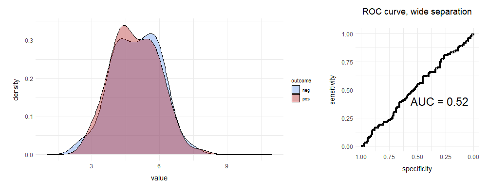
We randomly move either up or right, so we get a line that’s pretty much straight. This test fails to distinguish leopards from shadows. If you’re still a bit unclear, here’s a brilliant set of animations that illustrate the above concepts. If you’re interested in playing, I’ve provided the R code I used below.8
It’s clear that if the area under the curve (AUC, ‘C-statistic’) is close to 0.5, the test is rubbish; conversely a value of > 0.9 is usually considered excellent for most purposes, especially in clinical medicine.
Choose that cut
Even if we have an AUC of 0.92, this doesn’t tell us where to put our cutoff. This will depend. We’ll look into this and more in a subsequent post. But let’s keep things simple, for now.
In many circumstances, it seems reasonable to have a low threshold for detecting a ‘signal’. We’re up on the right of the ROC curve. Quite often, there’s a bigger down-side if we miss stuff, not just the lurking leopard, but also the presence of water or food or other people nearby, and so on. We can often compensate for a false positive, using further checks. This is actually how to do good Science. Make bold theories that are mostly wrong.⌘
The catch is that we will often make associations that just aren’t there. If we don’t or can’t check, we end up being misled. This may even be a compelling explanation for all sorts of strange human behaviours. These are not new ideas. In a 2006 paper, Haselton & Nettle argue that evolution may well have shaped us into being ‘paranoid optimists’. The obvious example they cite here is that men tend to overestimate women’s sexual intent; they also discover many other biases that fit.
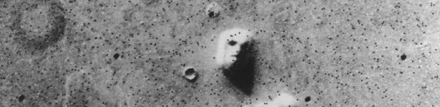
Indeed, we see this in a lot of human tendencies, for example the ‘face on Mars’ pictured above. In more detail, this is embarrassingly unfacelike. Similarly, we also quite often perceive causality that is just not valid.
And this brings us to the other, quite common case, where the test is just rubbish. The AUC is about 0.5. Here, it seems that we often resort to random pigeon religion.
So why?
Why do we succumb to quackery? We seem to have a built-in vulnerability—a tendency towards false positives—that can be compensated for by checking. But this can be subverted or deceived:
We may not know how to check. (How do I check a ‘face on Mars?’)
We may be so comprehensively deceived by a charismatic person that we fail to check. (“Don’t bother to check, I’ve researched this and I know.”)
We may even be prevented from checking. It’s blasphemous or illegal or dangerous to ask that question! (“Was Charlie Kirk not a good person?”)
We seem wired to make quick decisions that lead us in the direction of false positives.
This will leave us vulnerable in many circumstances.
In my next post, we’ll look at cases where ROC curves fail or are sub-optimal, and corresponding better options. We’ll also edge into the area of fraud and misuse of statistical tests by people out to make a quick buck. AI may feature prominently.
My 2c, Dr Jo.
⌘ This signifies one of my past posts where I explore the topic in more detail.
Body of collected knowledge about the therapeutic use of substances.
Not a monkey. As the L-space wiki points out about the librarian at Unseen University on the Discworld, who is an ape:
Anyone else using the m-word out of malice or willful ignorance is dealt with without mercy and shown an elementary biology lesson—ie, can a mere monkey hold somebody upside down by their ankles and bounce their head repeatedly off a hard unyielding floor?
We should also note that the authors didn’t try chewing or applying this herb themselves, to test whether it causes a discernible difference to e.g. wound pain.
Berberine and palmatine, as found in goldenseal, break DNA strands and cause liver tumours. The herbal ‘faithful’ seem to see ability to act like chemo as a positive feature of ‘herbal medicines’, without questioning whether unmonitored, unregulated, untested daily chemo is a wise choice for well people.
According to William L Ury in “Conflict Resolution among the Bushmen: Lesson in Dispute Systems Design” Negotiation Journal, October 1995, 379.
Here’s that cat analysis (unfortunately, MDPI). It’s obvious that a particular group of chimps may also refine their behaviour related to specific locations or plants. See later.
In fact, research in this domain gave rise to the first ROC curves.
Here’s my R code:
##########################
# install.packages('pROC')
# install.packages('patchwork')

library(tidyverse) # for bind_rows
library(ggplot2)

my_theme <- theme( plot.title = element_text(size = 18, hjust = 0.5),
            axis.title.x = element_text(size = 14, margin=margin(t=12)),
            axis.title.y = element_text(size = 14, margin=margin(r=12)),
            axis.text = element_text(size=12),
            plot.margin = margin(t=10, r=10, b=20, l=20)
          )

sep = 2  # Separation, use 0 for an AUC of ~0.5
neg <- rnorm(n=100, mean=5, sd=1)
pos <- rnorm(n=100, mean=5+sep, sd=1)
dneg <- data.frame(value = neg)
dpos <- data.frame(value = pos)
combo <- bind_rows(neg = dneg, pos = dpos, .id='outcome')
p_density <- ggplot(combo, aes(value, fill=outcome)) +
      geom_density(alpha=0.4) +
      xlim(1,11) +
      theme_minimal() +
      scale_fill_manual( values=c('neg'='cornflowerblue',
                                  'pos'='firebrick') ) +
        my_theme

p_density


### pROC provides ggroc() for ggplot functionality
#  [ otherwise need to pull out data and manually use ggplot() ]
#
library(pROC)
roc_out <- roc(combo$outcome, combo$value, levels=c('neg', 'pos'))
roc_out
## plot(roc_out)
p_roc <- ggroc(roc_out, colour='black', size=1.5) +
     theme_minimal() +
     coord_equal() +
     labs( title = 'ROC curve, wide separation') +
     annotate('text', x=0.30, y=0.4,
              label = paste( 'AUC =', round(auc(roc_out), 2)),
              size = 8
              ) +
     my_theme

p_roc

## side-by-side:
library(patchwork)

main_plot <- p_density + p_roc + plot_layout(widths = c(2, 1))

main_plot